

I Have 40 Columns Of Raw Data, How To Create A Template To Grab 10 Of Them?
Pivot tables are awesome! They're ane of Excel'south most powerful features, they allow you to quickly summarize large amounts of information in a matter of seconds. This collection of awesome tips and tricks will assistance you master pivot tables and go a data ninja!
You lot're gonna learn all the tips the pros utilize, so go set up for a very very long postal service!
Download the example file with the data used in this mail service to follow along.
Your Source Data Needs to be in Tabular Format
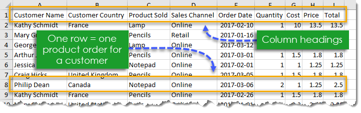
When using a pivot table your source data will need to be in a tabular format. This means your data is in a tabular array with rows and columns.
- The first row should contain your cavalcade headings which describes the data straight beneath in that column. There should be no bare cavalcade headings in your data.
- Each row later the column headings should pertain to exactly ane record in your data. For example, if your table contains customer data and so each row might have the name, street address, postal code and email address for exactly one client.
Apply a Table for Your Source Data
When creating a pivot table it's normally a skillful idea to turn your information into an Excel Table. When calculation new rows or columns to your source information, you won't demand to update the range reference in your pivot tables if your data is in a Table.

Without a table your range reference will look something like above. In this case, if we were to add data past Row 51 or Column I our pivot table would non include it in the results.
To create and proper name your table.
- Select your information.
- Go to the Insert tab and press the Table button in the Tables section, or use the keyboard shortcut Ctrl + T.
- Press the OK button.
- With the active cell inside the tabular array, go to the Table Tools Design tab.
- Change the Table Name under the Properties section and press Enter.
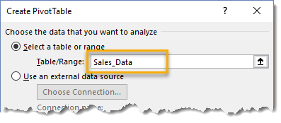
Now when you create a pin table yous tin reference it with a name instead of a range. When you lot add data to the table, you won't demand to update the range in your pin tabular array. Only refresh it and the new data will appear in your results.
Change Source Data
Ok, if you determine not to use a table for some reason, then you're going to accept to update the range when you add any new rows or columns outside the original range selected.
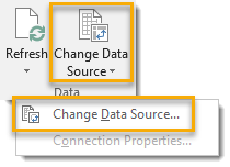
Select your pivot table and go to the Analyze tab and press the Change Data Source push then select Change Information Source from the menu. Update your range accordingly in the following Modify PivotTable Data Source pop upwards dialog box.
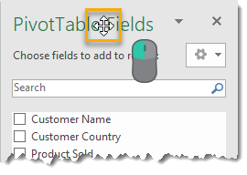
Undock the PivotTable Fields Window
To undock the PivotTable Fields window pane hover your mouse cursor over the title until it turns into a 4 way arrow, then right click and drag information technology to your desired location. You lot can either leave it floating somewhere in the spreadsheet or dock it to the left side by dragging information technology to the very left edge.
Rapidly Dock the PivotTable Fields Window
To quickly dock the PivotTable Fields window pane hover your mouse cursor over the title until it turns into a iv way arrow, then double right click. It will dock to the last docked location (either to the right or left side).
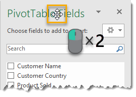
Hide or Unhide the PivotTable Fields Window
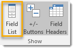
You lot tin can get more than screen existent estate by hiding the PivotTable Fields window. Select a jail cell in your pivot tabular array and and then get to theAnalyze tab in the ribbon. Printing the Field List button in the Prove section to toggle the PivotTable Fields window on or off.
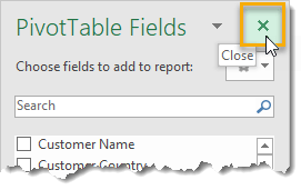
You can also close the window using the Ten in the upper correct corner.
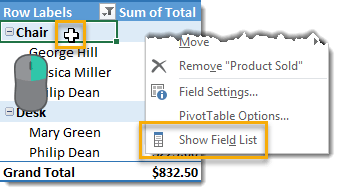
You tin as well show or hide the PivotTable Fields window with a right click anywhere within your pivot table then select Bear witness Field Listing or Hide Field Listing (depending on the current state of your PivotTable Fields window).
Alter the Default Arrangement of the PivotTable Fields Window
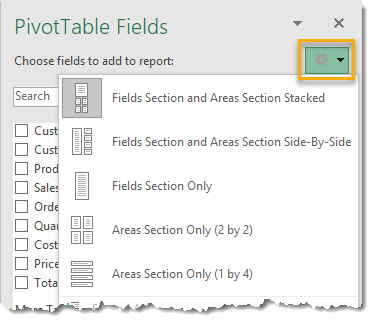
Click on the gear bicycle with a downwardly arrow to modify default appearance of the PivotTable Fields window.
There are five dissimilar available options you lot can select from.
- Field Department and Areas Section Stacked
- Field Department and Areas Section Side-By-Side
- Field Department Merely
- Areas Section Only (2 by 2)
- Areas Section Only (1 by four)
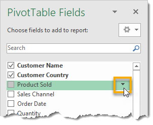
Change the Sort Order of Your Field Listing
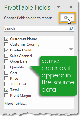
The list of data fields will show in the same order as the source data by default. Y'all tin change this to show in alphabetical gild (A to Z) if yous prefer. Left click on the options carte du jour in the PivotTable Fields window to access the option.

Select the Sort A to Z option in the menu. Your fields will now brandish in descending order!
Motion, Resize and Close the PivotTable Fields Window
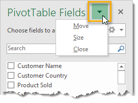
Right click on the small downward arrow to the correct of the PivotTable Fields title to motility, resize or close the window.
- Move – This volition allow you to undock the window and movement it around the spreadsheet.
- Size – This allows you to adapt the width and height (when undocked) of the window.
- Close – This allows you to close the window. Y'all can open up information technology again from the Analyze tab > Field Listing command.
PivotTable and PivotChart Wizard Keyboard Shortcut
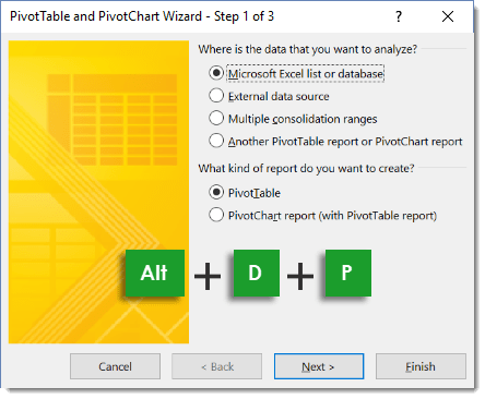
Apply the keyboard shortcut Alt + D + P to open up the PivotTable and PivotChart Wizard. This volition take you lot through the steps to fix either a pivot table or pivot chart, select your data and the location for your new pin table or chart.
Create a PivotTable With a Keyboard Shortcut
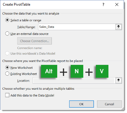
Apply the ribbon command keyboard shortcut Alt + North + Five to quickly create a pivot tabular array.
Show Details Backside a Value
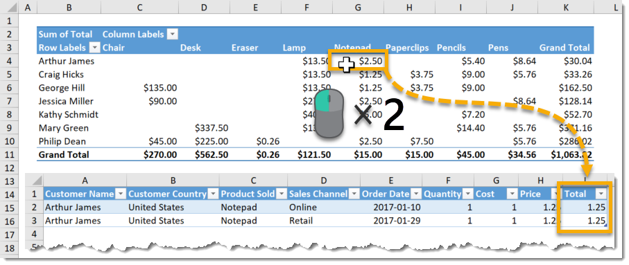
Double correct click on a value inside a pivot table to quickly see the data backside that aggregated value. A new sheet volition be created with only the data relating to that value.

Y'all can too admission this feature by correct clicking on any value and so selecting Testify Details.
Turn Off Evidence Details to Avoid Accidental Double Click
If the power to show the detailed data backside a pin table result doesn't involvement y'all, and then yous can turn this feature off. This means you and tin can avoid creating new sheets with bits of data in them because of adventitious double clicks.
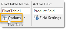
Select your pivot tabular array and go to the Analyze tab in the ribbon. Press the Options button in the PivotTable section to open up the options menu.
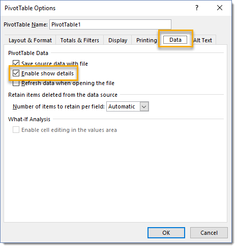
In the PivotTable Options carte go to the Information tab and uncheck the Enable show details box to disable this feature.
Replace Blank Cells
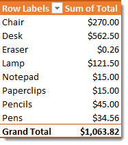
This pivot tabular array contains blank cells because our source data does not comprise whatever records for those combinations of dimensions. For instance, there is no data for Arthur James and France then the intersection of the Arthur James row and France cavalcade is bare. We tin can change the settings to display something such as a nada or some text saying "N/A" instead of a bare.
Left click anywhere in the pin tabular array then select PivotTable Options.
In the PivotTable Options menu
- Get to the Layout & Format tab.
- Bank check the For empty cells bear witness box and enter the value y'all would similar to show for blanks. In our example we will supersede blank cells with 0.
- Printing the OK push button.
Now the previously blank cells accept been replaced past zeros.
Show Items with No Data
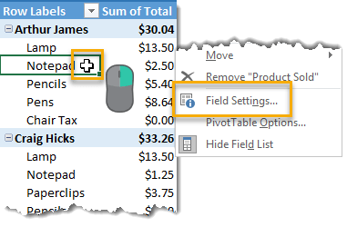
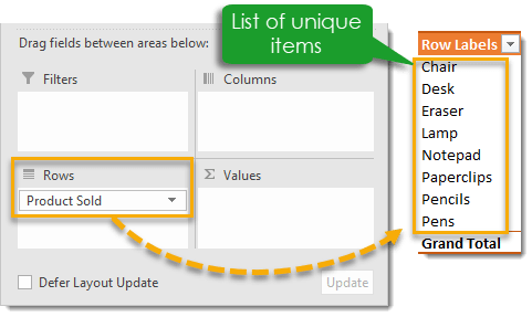
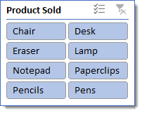
In this example nosotros have create a pivot tabular array with Customer Name and Production Sold in the Rows area. Find that under each client, not all the possible products are listed. Merely those which we have a transaction in our information are listed. We can modify this so that nosotros encounter all items even when there is no data.
Right click and select Field Settings from the menu.
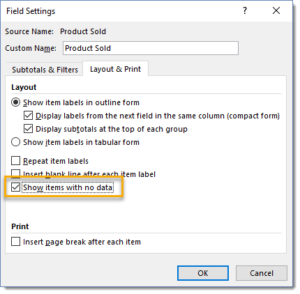
Check the Show items with no data box and press the OK button.
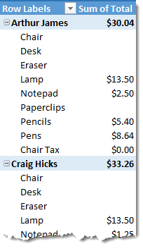
Now we can see all the available items in the Product Sold field even when there is no information.
Remove Items from a Filter Using a Keyboard Shortcut

Highlight items in a row or cavalcade and press Ctrl + – to remove them from the filter. You tin can select non-adjacent cells past property Ctrl and so clicking on the cell.
Add the Current Selection to the Filter
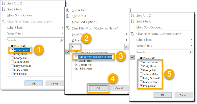
Yous tin can use the Search from within a pin table filter to add items to your previously selected items. This is substantially like using an OR condition in your filtered item searches.
- Select your beginning set of items to be filtered on either manually or using the search box (with the aforementioned method as step 2 & 3).
- Apply the Search box to search for and then select the second set of items to exist filtered on.
- Check the box marked Add current selection to filter that volition announced when using the search box.
- Press the OK button.
- At present if yous view the filter, you will see both your selections from step i and selections from step ii included in the filter.
Use the Select All Filter Toggle
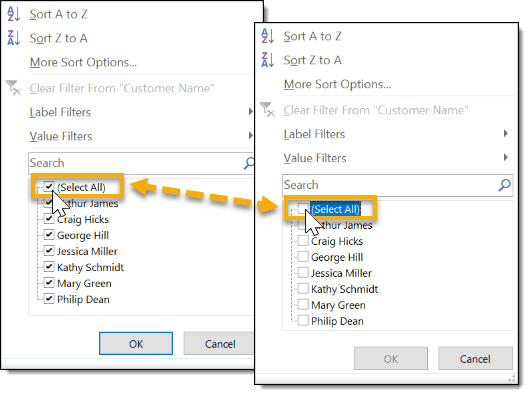
Rapidly select or deselect all items in the filter past using the Select All filter toggle. This can be very handy when dealing with a long list of items. Yous tin can quickly deselect all and then manually select a small-scale number of items or apace select all and manually deselect a minor number of items.
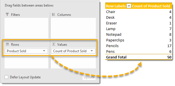
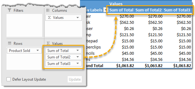
Defer Layout Update
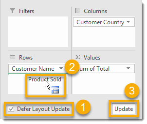
You can defer updating the pivot table while yous make changes in the PivotTable Fields window. This is by and large only useful if your table is connected to a very large data source and you need to make many changes to the layout. This option is more than useful for connections to external data sources equally pivot tables with any data you tin fit into Excel should be pretty responsive.
- Cheque the Defer Layout Update box in the PivotTable Fields window.
- Make the changes to your layout in the Filters, Columns, Rows or Values section. Your pivot table will remain static.
- Press the Update button and your table will update to reflect all the changes made.
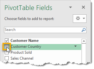
Add together or Remove Fields Using the Cheque Box
You can quickly add fields to your pivot tabular array by using the cheque box next to the field name from the field list in the PivotTable Fields window. This can save time if you take a lot of fields to add together instead of dragging and dropping each item. Fields containing text data volition be added to the Rows section and fields containing numeric data volition be added to the Values section when using the check box.
Filter Fields from the PivotTable Fields Window
You can filter items in a field from the field list in the PivotTable Fields window. The filter volition only use when the field is added to the filters, columns or rows area. Hover over the desired field and click on the small downward arrow to the right of the field name to open up the filter carte.
Rename Any Label

You can rename whatsoever label in a pivot tabular array merely by selecting the cell and typing over it. You can modify particular names in a field, row headings, column headings, filter labels, totals or thousand full labels. The only weather are you lot tin can't rename it to something that already exists in your source data and you lot tin can't blazon over a value. This doesn't alter the source data, information technology just changes how the item is labelled.
Rename A Label With A Trailing Space

Ane thing you may want to exercise is alter a column heading like our "Total" cavalcade that appears as "Sum of Full" to just show "Total" in the pivot table. Unfortunately, this can't be done, since "Total" already exists in the source data. If you try to practise this y'all will get a warning pop upwards saying "PivotTable field proper noun already exists". Nosotros can get around this past adding a space graphic symbol to the end of the proper name. This will count as a different name just visually it volition look the same as the former field name.
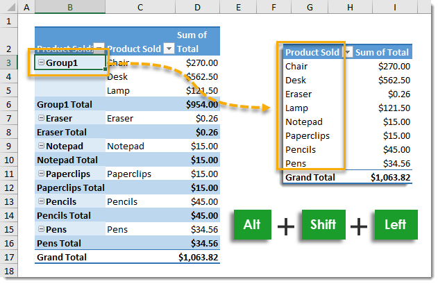
Grouping Together Items in a Field
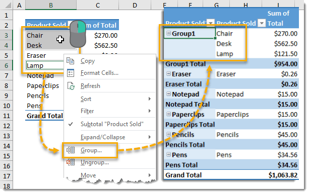
You lot tin group items in a field together to farther summarize your information. Highlight the items and and so right click and select Group from the menu. Y'all can select multiple non-adjacent field items by belongings the Ctrl cardinal while making your selection. By default, the grouped name for a set of items will be Group1, Group2, Group3 etc… But you tin modify these to something more meaningful.
You tin can too ungroup a grouped field. Select it and right click then choose Ungroup from the menu.
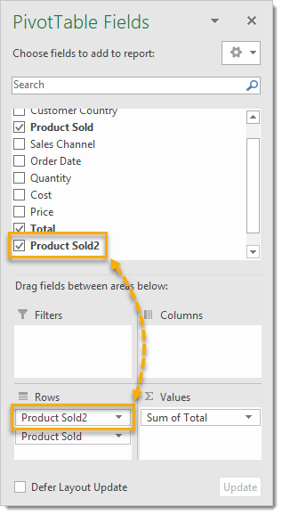
You will find a new field in appear which has the aforementioned proper name as the grouped field but with a number appended to the end. This is the newly created grouped field and you can utilise it just like any other field in your data. You can move it to the Filter, Row, Cavalcade area or remove it completely from the pin table. Note that removing it from the pivot table will not ungroup the field.
Group Together Items in a Field Using a Keyboard Shortcut
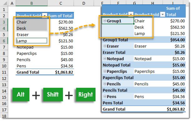
You tin can quickly group together items in a field past highlighting the items you want to group then pressing Alt + Shift + Right Arrow central.
Ungroup Grouped Items Using a Keyboard Shortcut
Yous can speedily ungroup grouped items by highlighting the grouped item and so pressing Alt + Shift + Left Arrow central.
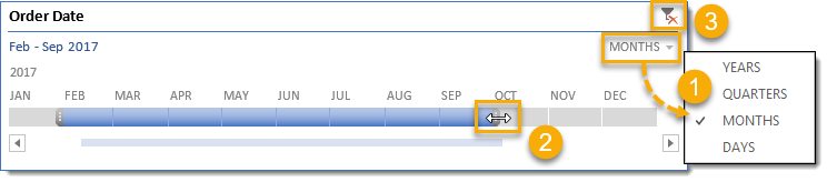
Group Dates
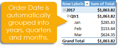
Group dates works a petty differently than group items in a field. When yous add a date field into either the rows or columns area, Excel will assume y'all probably want to view the information by Month, Quarter or Year and will automatically group the dates similar this. If y'all actually wanted the view by appointment, you lot will need to right click on it and choose Ungroup from the carte du jour.
I've added the Order Date into the rows area and nosotros can run into information technology'southward been grouped by year, quarter and month.
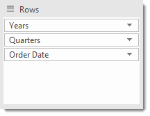
Just similar when grouping items in a text field, Excel creates new fields which tin can be use similar any other field. You tin remove the original date field without affecting the year or quarter fields.

When you right click on the date field and select Group from the menu, you will exist presented with a variety of group options.
- You can choose the Starting and Ending dates. All other dates exterior the range will be bucketed into a group less than the start engagement and a group greater than the end appointment.
- Choose the levels of granularity for your grouping.
- If you select only Days as the group, you can cull to group based on the Number of days. Choosing 7 would be equivalent to group by weeks.
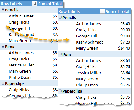
Grouping Numbers into Ranges
Excel can also grouping numerical fields. This can be handy if you lot want to know something similar "How much of my sales are from orders less than $50?".
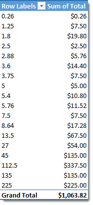
If I place the Full field in both the Rows and Values area, I don't get anything that useful.

If y'all correct click on the row, this numerical grouping menu volition open and y'all can select a Starting and Ending point forth with the interval length.
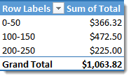
Now it'southward easy to see what range most of the sales are in.
Search the PivotTable Fields List
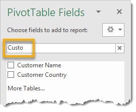
If your source data has a lot of fields and so using the search box can help to narrow downward the list to find what yous're looking for.
Give Your Pivot Table a Different Style
Speedily modify the style of any of your pin tables using the preset PivotTable Styles.
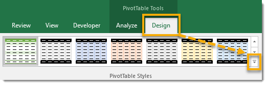
Get to the Design tab in the ribbon and click on the pocket-size downward arrow in the PivotTable Styles section to reveal a total choice of pivot table styles available. Note, the Blueprint tab is only visible when the active cell cursor is in a pivot tabular array.
Explore Different Style Options
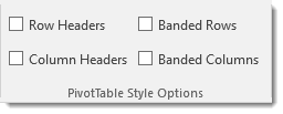
Toggle different PivotTable Fashion Options on or off. Become to the Design tab in the ribbon and look for the PivotTable Manner Options department.
Each choice tin can be independently turned on or off to add together a particular way chemical element to your pivot table.
- With all options unchecked the pivot table is empty of row headers, banded rows, column headers and banded columns.
- Adding Row Headers.
- Calculation Banded Rows.
- Adding Column Headers.
- Calculation Banded Columns.
Refresh Your Data
You will demand to refresh your pivot table when you add to or change your source data if you lot want to encounter these changes reflected in your pivot table results. You can exercise this from several locations.
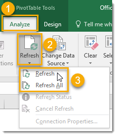
Select a prison cell in your pivot table to activate the PivotTable Tools tabs.
- Become to the Analyze tab.
- Press the Refresh push.
- Select either Refresh or Refresh All.
- Refresh will refresh any pivot table continued to the source data of the active pivot tabular array.
- Refresh All will refresh all data connections for all pin tables in the workbook.
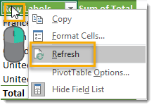
You can besides refresh with a Right Click anywhere inside a pivot table and selecting Refresh from the menu.
Refresh with a Keyboard Shortcut

Refresh the connexion to the active pivot table's source data by using the Alt + F5 keyboard shortcut.
Refresh All with a Keyboard Shortcut

Refresh All information connections for all pivot tables in the workbook past using the Ctrl + Alt + F5 keyboard shortcut.
Automatically Refresh Information when Opening Your Workbook
If you want to make sure you're e'er looking at the latest data in your pivot tables, you can set the workbook to refresh all pivot tables connected to particular data source. This is especially useful with external data sources.
Select i of the pin tables continued to your data source then get to the Analyze tab and press the Options button institute in the PivotTables section.
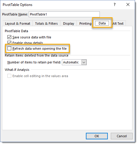
From the PivotTable Options menu, go to the Data tab and check the Refresh information when opening the file box. This will refresh all pivot tables in the workbook which are connected to the same data source.
Select the Entire Pivot Tabular array
If yous're like almost people, you lot'll probably stop up making several copies of a pivot tabular array in order to have different views of the data at the same time. If your pin table is large or has items in the filter expanse, information technology can be tricky to select all of it in order to copy and paste. This is when Select Entire PivotTable comes in handy.

Go to the Analyze tab and press the Select command under the Actions section then choose Entire PivotTable. This volition select all of the pivot table including any filter elements higher up the table.
You tin can also choose to select merely the Labels or the Values area from here.
Clear All Filters
If you have multiple filters engaged on your pivot table y'all tin chop-chop clear them all without going into each individual filter menu and selecting the Articulate Filter From option.
Select a cell in the pivot tabular array which you want to clear filters from to actuate the PivotTable Tools tabs in the ribbon.
- Become to the Analyze tab.
- Printing the Clear button from the Deportment department.
- Select Clear Filters from the menu.
Your pivot table volition revert back to a completely unfiltered state showing results based on all source information.
Clear Your Entire Pivot Tabular array
You can articulate your pin tables entirely back to the initial blank country if you want to start over completely with your pin table analysis.
- Go to the Analyze tab.
- Press the Articulate button from the Actions section.
- SelectClear All from the menu.
Your pin table will now be in its initial blank land with all fields and filters removed.
Clear One-time Field Items
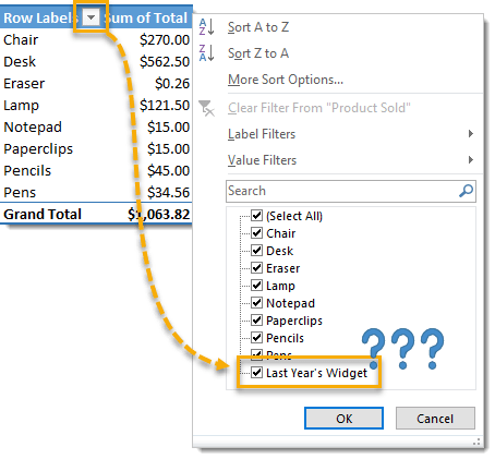
You might have seen this happen earlier. Y'all delete sometime data and so add in the new information, but you still see items from the quondam data subsequently you refresh the pin table. These items are still stored in the pivot cache and displayed in filter selections fifty-fifty if there is no information for information technology at all. Information technology can be very confusing when information technology happens.

You tin change the settings so that your pivot cache doesn't retain any of the old field items when y'all refresh your data. Go to the Analyze tab and press the Options button found under the PivotTable section to open up the PivotTable Choice. So become to the Data tab and select None under the Number of items to retain per field option.
Now when you refresh, the old phantom items will no longer appear.
Format Numbers
Unfortunately, number formatting from source data does non transfer into your pin tables. Y'all may want to format your numbers to make them more than readable.

To format a given field, Right Click on any number in that field and select Number Format from the carte du jour. The familiarFormat Cell dialog box volition open up with only the Numbers tab available and you lot will be able to format the numbers in your field the same as any other jail cell in your workbook.
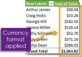
The cool thing is that applying your number formats this way will exist dynamic. Even when you motion the field effectually in the pin table, add other fields or filter on items the formatting will remain practical to the entire field in the pivot table.
Expand or Plummet Field Headings
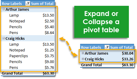
If your pivot table has multiple dimension fields in a row or column you can expand or collapse the outer fields to prove more than or less detail.
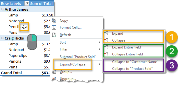
Right click on the field you lot want to expand or collapse and select Expand/Collapse from the card.
- Y'all can aggrandize or plummet only the selected item and leave the remaining solitary.
- You lot can aggrandize or collapse every detail in the field selected.
- You can expand or collapse only the selected detail to a given level.
Double Click to Aggrandize or Collapse Field Headings
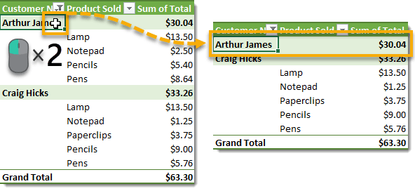
You tin aggrandize or plummet fields with a double right click on the field item. This is great to de-clutter a pivot table when you only need to show the total detail for one item.
Add or Remove Aggrandize or Collapse buttons
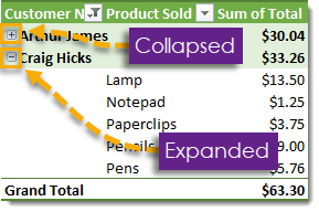
Y'all can add expand or collapse buttons to your pivot tables to arrive more obvious to another user that they can expand or collapse the pivot table view every bit well as which items are already expanded or complanate.
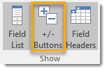
To add together these buttons, select your pin table and get to the Clarify tab and press the +/- Buttons push in the Show section.
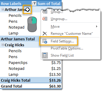
Automatically Create a Pin Table for each Item in a Filter
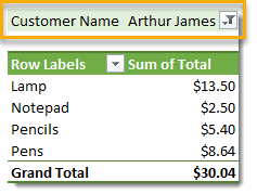
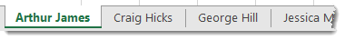
Let's say yous have a pivot table with a field in the Filter area and y'all would similar a pivot table for each particular in the field. You might retrieve this has to be washed manually by copying the pivot tabular array and so filtering on a new particular in the field, but this tin actually exist washed automatically using Testify Report Filter Pages. In our example we accept the Customer Name field in the filter area and pivot tabular array is currently filtered on Arthur James, and nosotros desire a pivot table like this for each customer.
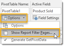
Select you pivot table, it will demand to have a field in the filter area. Go to the Analyze tab in the ribbon and press the Options button found in the PivotTable section so select Testify Report Filter Pages from the card.
Select the desired field from the Show Report Filter Pages dialog box if you have multiple fields in the filter surface area of your pivot tabular array then press the OK push.
Excel will now create a new sheet for each item in the field you selected. Each sheet will be named after the item in your field and will comprise a copy of your pivot table filtered on that detail. It's a big time saver when you accept a lot of items in your field.
Allow Multiple Filters Per Field
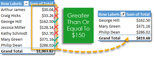
Excel has two types of filters bachelor for a pivot tabular array field, Characterization Filter and Value Filter. Permit's say you wanted to filter this pivot table on all Product Sold that get-go with "P" (using a Label Filter) and having a Total value larger than $20 (using a Value Filter), with the default settings this is non possible to have both filters at the same fourth dimension. We tin can update the settings to permit this.
Select your pivot table and go to the Analyze tab in the ribbon and press the Options button in the PivotTable department.

Enable multiple filters in the PivotTable Options dialog box.
- Go to the Totals & Filters tab.
- Cheque the Allow multiple filters per field box.
- Press the OK button.

Now you lot will be able to use both Label Filter and Value Filter at the aforementioned time on i field.
Go a List of Unique Values from a Field
You can use pivot tables to get a list of the unique values in any field of your data. Simply drag the field which you want unique values from into the Rows area of a blank pivot table and the resulting pin tabular array will comprise a list of unique values from your data for that field.
Count the Occurrence of an Item in a Field
Placing any field with text information into the Values area of the pivot tabular array will cause the adding to default to Count instead of Sum. This ways nosotros will go the count of the number of occurrences of each detail. In this instance, nosotros have placed Product Sold field which contains text data, into both the Rows and Values area of the pivot table, and we see Count of Product Sold in the Values area.
Delete Your Source Information
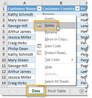
After creating your pivot table you can delete the source data if you desire to reduce the workbook file size. You lot can delete your source data by deleting the sheet it's contained on. Right click on the sheet tab and select Delete from the menu. Your pin table contains a cache of the data and then information technology will keep to work as normal. If you desire to see your data again you tin double left click on the one thousand total of your pivot table and the data will appear in a new sheet.
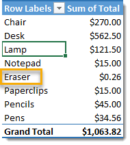
Sort Items Alphabetically in Ascending or Descending Order
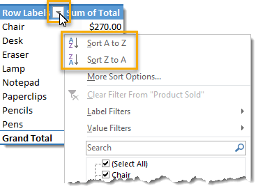
Sort items alphabetically in either ascending or descending gild. Left click on the filter icon and select Sort A to Z for ascending or Sort Z to A for descending club.
Manually Sort Items
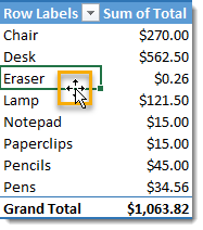
Select the particular you desire to move and hover your mouse cursor over the active jail cell border until it turns to a four-way arrow cross.

Left click and drag the item to its new position. You will run across a big light-green bar that indicates where the detail will be placed.
Release the detail into its new position.
Sort Items According to a Respective Value
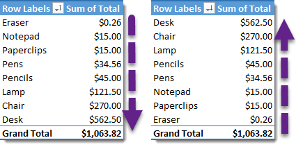
You can sort your pin table by ascending or descending values.
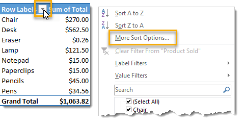
From the filter menu select the More Sort Options.
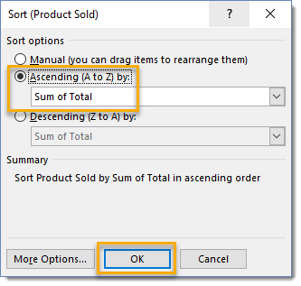
Select either Ascending (A to Z) or Descending (Z to A) and so choose one of the value fields in your pivot table and so press the OK button.
Create a Custom Sort Order
If sorting a field alphabetically in ascending or descending order doesn't suit your needs, you can create a custom sort lodge by creating a custom list!
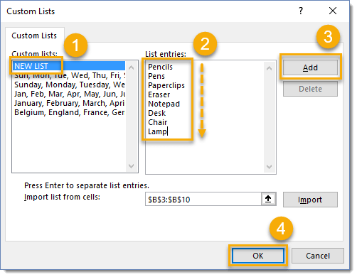
To add together a custom list, go to the File tab in the ribbon and select Options. From the Excel Options card choose Advanced then ringlet downward to the General section and printing the Edit Custom List button.
- Select NEW LIST from the Custom lists box.
- Enter your list of field items appearing in the order you lot want them to sort in your pin table.
- Press the Add push button to add your list.
- Press the Ok button.

Refresh your pivot table and the gild volition change to that of the listing you entered. This volition as well be the default sort society at present for that field any time you create a pivot table with that field in it.
Insert Blank Line After Each Particular
For a less cluttered look and feel you can insert a blank line subsequently each item in your pin tabular array. Select your pivot table and go to the Blueprint tab of the ribbon and click on the Blank Rows push in the Layout department and then select Insert Blank Line afterwards Each Particular.
Items in your pin table will be visually separated with white space so the viewer knows that the data pertains to something unlike. You tin can become rid of these blank rows from theDesign tab of the ribbon and clicking on the Blank Rows button in the Layout section and then selectingRemove Blank Line later on Each Detail.
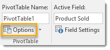
Double Click to Open Value Field Settings
You can double correct click on any cavalcade heading to open the Value Field Settings for that field.
Count Distinct Items
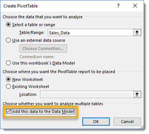
To count distinct items you will need to create your pin table with information added to the Data Model. Bank check the Add this information to the Data Model box when creating your pivot table.
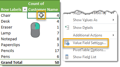
In this example, we take our Product Sold field in the Rows area and Customer Proper noun in the Values area which gives the states a count of the orders by product. If we want a unique count of the customers who ordered each of the products and so we need to change the default Count to Distinct Count for our values settings.Right click anywhere on the field which you want to obtain a distinct count for and then select Value Field Settings from the card.

From the Value Field Settings select Distinct Count to summarize value field by and press the OK push.
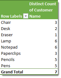
Now the values volition display the distinct count. Note the Thou Total at present reflects that we have 7 singled-out customer names in our data of 50 orders.
Hide Selected Items

You tin can hibernate selected items quickly without going into the filter menu (small down pointer side by side to the column heading).
- Select the items you want to hide with your filter. You lot can utilize Ctrl to select non-next items. Then correct click on the selected items.
- Select Filter from the carte.
- Select Hibernate Selected Items from the sub carte.
This allows you to quickly filter out items without going into the filter menu and checking or unchecking boxes in a long list of items.
Keep Selected Items
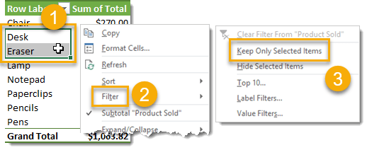
Similarly to hiding selected items, you lot can choose to keep merely the selected items with a filter.
- Select the items you want to continue with your filter. You can apply Ctrl to select non-side by side items. Then right click on the selected items.
- Select Filter from the menu.
- Select Go on Simply Selected Items from the menu.
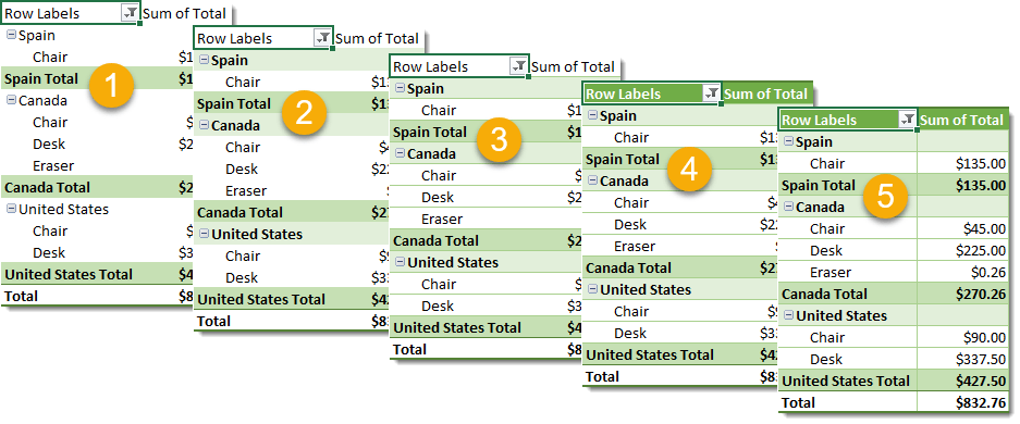
Alter the Layout
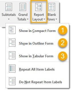
To change the layout of your pivot table go to the Design tab and select Report Layout push button under the Layout section. Y'all tin select from three different layout options.
- Show in Compact Course
- Evidence in Outline Form
- Show in Tabular Form

To demonstrate the different layout options, we have created a pivot table with ii fields (Product Sold and Customer Name) in the Rows section and a field (Total) in the Values section.
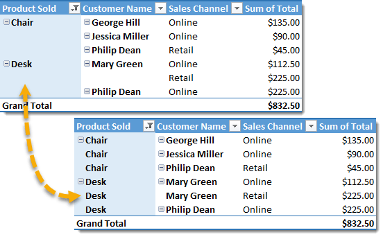
- Meaty form will contain all the Row fields in one column in a hierarchical construction.
- Outline class will yet have a hierarchical structure only each Row field will be in a separate column in the pin table.
- Tabular grade will not be in a hierarchical structure and each Row field will be in a split up column in the pivot table.
Repeat All Item Labels
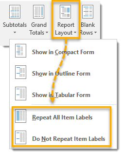
You can repeat all your pivot tables item labels by going to the Blueprint tab and selecting theStudy Layout button under the Layout department. Select Repeat All Item Labels to turn on repeated labels and select Do Not Repeat Item Labels to turn off repeated labels.
Past default, a pin table will show the field label so blank cells underneath for all other sub-fields included in the field heading. Creating a Tabular Form layout with Repeat All Item Labels is a great way to create some other set of more aggregated "Source Data" that you can copy and paste every bit values and utilize elsewhere.
Turn Thousand Totals On or Off
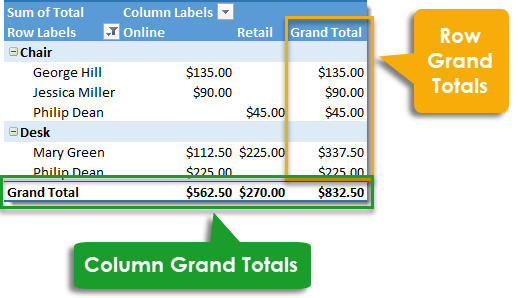
You can add grand totals to your pivot table to help you come across at a glance the total for any values field across any row or column.
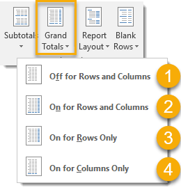
Get to the Design tab and select the Grand Totals command from the Layout section. Select from the four choice for displaying thou totals.
- Off for Rows and Columns (no grand totals will brandish)
- On for Rows and Columns
- On for Row Only
- On for Columns Only
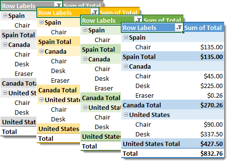
Plough Subtotals On or Off
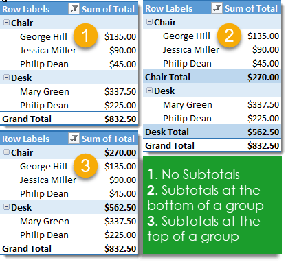
When your pin table has more that one dimension, you tin can add or remove subtotals to make results easier to understand.
- No subtotals results in a cleaner looking pivot tabular array, but you lose vital information about totals beyond parent level field grouping.
- Adding subtotals beneath the group results in actress rows in your pivot table.
- Adding subtotals higher up the group results in the actress data but without the actress rows (with a meaty layout).
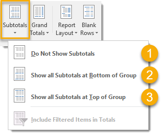
Get to the Design tab and select the Subtotals command from the Layout department. Select from three option for displaying subtotals in your pivot table.
- Practice Not Show Subtotals
- Show all Subtotals at Bottom of Group
- Show all Subtotals at Height of Group
Plough Off GETPIVOTDATA
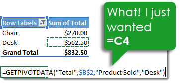
Past default when yous try to reference a cell inside a pin table in a formula, Excel will create a GETPIVOTDATA formula for the reference. These tin can be abrasive when you want a unproblematic relative A1 style reference since the GETPIVOTDATA acts similarly to an absolute reference.
You can turn this default option off by selecting your pivot table and so going to the Clarify tab in the ribbon and clicking on the small downwards arrow next to the Options button under the PivotTable section. Uncheck the Generate GetPivotData option to turn this feature off. You can also plough it back on from there too!
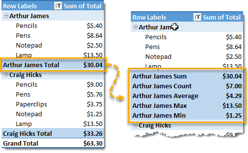
Add together a Second Field to the Values Area
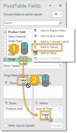
You lot tin can add the aforementioned field to the Values area of your pivot table two or more times.
- Right click on the field yous desire to add to the Values area again and select Add to Values.
- You tin can as well left click and drag the field into the Values surface area again.
Each time you add the field to the Values surface area it will get a sequential number added to the end, but remember y'all can modify these titles. You lot can and then change the summarize type to testify a Count, Average, Max, Min, Variance or Standard Divergence instead of the Sum. This will allow you lot to summarize the field in a diversity of different ways at the aforementioned time.
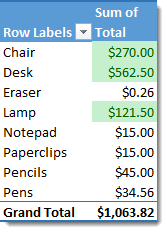
Add together Data Confined
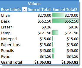
Calculation data bars can be a bang-up way visually show the relative value of each item in your pivot table. In the above table we've added the Total field to the pin table twice and used one instance to add data bars to the pivot table.
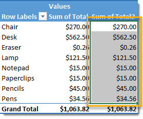
Select the range in your pivot table where yous'd similar to add the data bars.
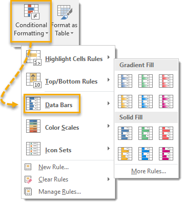
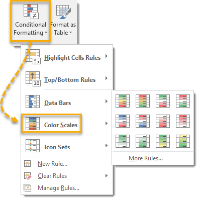
Go to the Home tab in the ribbon and under the Styles section press the Conditional Formatting button and so select the Data Confined option from the carte du jour. You can cull either a Gradient Fill or Solid Make full and there are several different color options available. You can besides create your own style data confined using the More Rules options in the carte. The cool matter is these data bars will be dynamic and applied to the unabridged field even if the range changes when you add together dimensions or update data.
Add Colour Scales
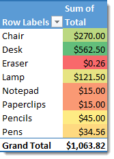
Y'all tin can add colour scales to your pivot tabular array to create a heat map to easily identify high, medium and depression values in your information.
Select the range in your pivot table where you would like to add the color scales.
Go to the Habitation tab and under the Styles section press the Conditional Formatting push button and then select the Color Scales option from the carte. There are several different color options to choose from or you can create your own rules and color options by selecting More than Rules.
Add Icon Sets
Y'all can add diverse icon sets to your pivot tables to visually betoken items that increased, decreased or stayed the same.
Select the range in your pivot tabular array where you lot're wanting to add together the icons.
From the Home tab and in the Styles section press the Conditional Formatting push so select the Icon Sets option. You'll find a large variety of icon options to cull from including arrows, shapes, flags, checks and Ten's, stars and many others. You lot can adjust the rules for when each symbol appears by using the More Rules option.
Add Highlighted Cells Rules
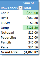
You tin can add conditional formatting to highlight prison cell values that fit certain rules to make them stand out. In this example I have created a rule to highlight cells betwixt $100 and $300. You can create many different types of rules.
- Numbers greater than a given value.
- Numbers less than a given value.
- Numbers between ii given values.
- Numbers equal to a given value.
- Text that contains a specific string.
- Dates that run across a given criteria.
- Indistinguishable values.
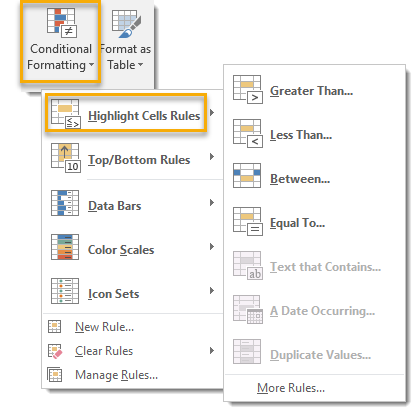
Go to the Dwelling house tab and in the Styles section select Conditional Formatting then select the Highlight Cells Dominion pick. You tin can and so select from the options mentioned higher up and set the criteria values required.
Add Highlighted Acme or Bottom N Formatting
You can add conditional formatting to highlight cells that are in the elevation N or bottom Northward values of the pin table. In this example I have added the formatting to show the top 3 values. Choose from several unlike options.
- Top 10 items.
- Top 10 percent.
- Bottom x items.
- Bottom x pct.
- To a higher place average.
- Below boilerplate.
Although these options mention top and bottom 10, the number can be selected as desired.

In the Home tab and under the Styles section select Conditional Formatting then select the Tiptop/Bottom Rules option. You can then select from the options mentioned above.
Format Numbers every bit Invisible Text
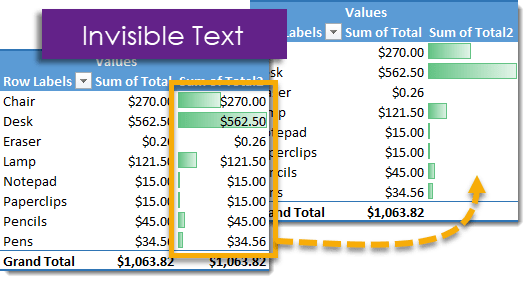
If you've added some sort of conditional formatting like information bars to your pivot table and want to get rid of the numbers to clean up the wait of the table, then yous can format the numbers every bit invisible text.

Right click anywhere in the field which you desire to format and select Number Format from the menu. In the Format Cells dialog box choose Custom from the Category so type 3 semi-colons ;;; into the Type surface area and press OK. The data volition nonetheless exist in your pivot table, just information technology just won't be visible!
Use Conditional Format Settings to Remove Text
When yous add together data confined or icon sets with conditional formatting, there is actually a setting to show only the data confined or icons. This tin be constitute in the More Rules carte du jour when setting up your provisional formatting.
This is a more simple choice than messing around with custom formats, but is express to data bars and icons.
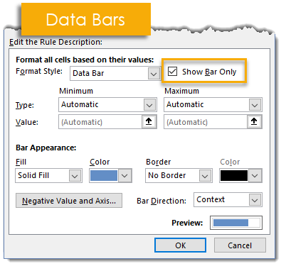
For the data bars bank check the Bear witness Bar Just box.
For the icon sets cheque the Bear witness Icon Only box.
Prevent Column Width Changing on Update
By default Excel will automatically adjust columns of a pivot table so that everything fits. This ways those really long headings like Count of Customer State will have upwardly a lot of column space. If y'all adjust these wide columns to a smaller size, the next time you update the pin table they will machine adapt back to fit the long heading title. Y'all can change the settings and then this doesn't happen.
Open up the pin tabular array option. Select your pivot table and go to the Analyze tab in the ribbon then press the Options button in the PivotTable section.
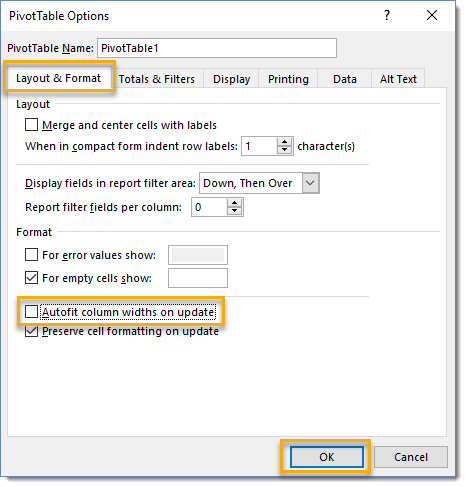
In the PivotTable Options window under the Layout & Format tab uncheck the Autofit cavalcade widths on update box. This will allow you to make changes to your pin table without the column width automatically adjusting.
Add together A Calculated Field
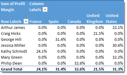
Calculation a calculated field to your pivot table is equivalent to adding a new column to your source data to perform a calculation based on the other data. For case, our data contains a Total Price and Full amount for each order. If we want to summate the Profit Margin on each order nosotros could add together another cavalcade with the adding Profit Margin = i – (Full Cost / Full) or we can add calculated field.
For a charge per unit type calculations similar a turn a profit margin, it's ameliorate to add the calculations as a Calculated Field rather than add an extra column with the calculation to the source data. Adding a rate adding to the source data may result in incorrect calculations in your pivot tabular array when viewing a pivot tabular array at a more than aggregated view than the data. Always add a calculated field instead!
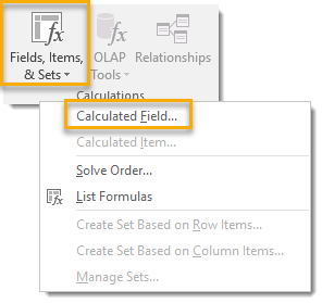
Select your pin table and go to the Analyze tab in the ribbon and press the Fields, Items & Sets push found in the Calculations section. Then select Calculated Field from the menu.
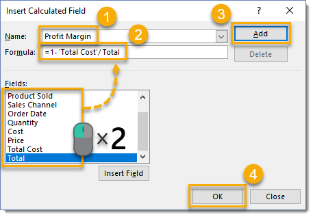
Add together your calculation in the Insert Calculated Field dialog box.
- Give your new calculation a Name. This is the field name that will appear in the pivot tabular array.
- Create your Formula. You can double right click any field in the field list to use it in your calculation.
- Press the Add together button.
- Press the OK push.
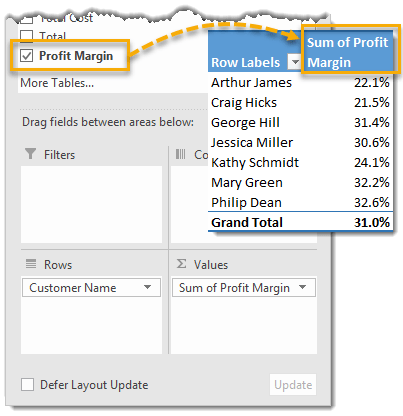
Your calculated field will announced in the PivotTable Field list and tin can be used to create your pin table just similar any other field.
Removing A Calculated Field
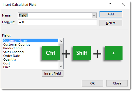
You can delete a calculated field past selecting your pin table past going to the Analyze tab in the ribbon and pressing the Fields, Items & Sets button so selectingCalculated Field from the card.

Delete a calculated field from the Insert Calculated Field dialog box.
- Use the drop downwards carte to select the calculated field you want to delete.
- Press the Delete button.
- Printing the OK push.
The calculated field volition no longer bear witness up in your PivotTable Field list. Note, this can't be undone!
Insert a Calculated Field with a Keyboard Shortcut
You tin can quickly open the Insert Calculated Field dialog box to create a new calculated field or edit an existing calculated field by using the Ctrl + Shift + + keyboard shortcut.
Add a Calculated Item
If adding a calculated field is like adding a new column to your source data, then adding a calculated particular is like adding a new row.
Let's say we have a simple table set that shows the product sold along with the full sales. Our Total column in the data doesn't include any revenue enhancement, just there is a 15% chair tax we need to include in our analysis. No problem, we can add this with a Calculated Particular!
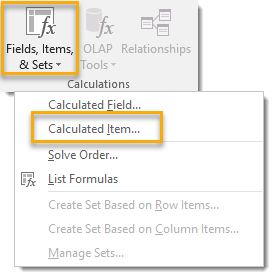
Select a field cell in your pivot table (the calculated detail option volition be grayed out if you lot select a value cell). Go to the Analyze tab then press the Fields, Items & Sets button in the Calculations section. Select Calculated Item from the menu.
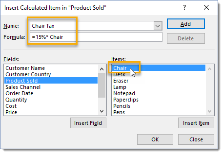
Give your new calculated row a name, then add in a formula. You lot tin can add together an particular into the calculation past selecting the advisable field then double clicking on any of the items in the field or pressing the Insert Item button.
I named the calculation Chair Taxation and the formula will calculate 15% of the value being summarized.
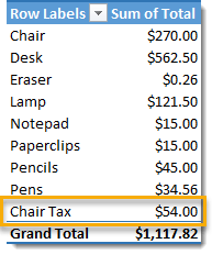
Nosotros at present come across a new row chosen Chair Revenue enhancement announced in our Product Sold field and the value is fifteen% of the Chair value. Annotation that this new row does contribute to the one thousand total.
Replace Errors

If you lot create a calculated field with a division operation like our profit margin calculation, so information technology's possible you might run across some #DIV/0! errors (divide by nil). Y'all can supercede these with a number like 0 or some text of your choosing to brand the table more presentable. Seeing these errors won't instill conviction in your audition, then information technology's best to replace them with something more assuring.
Select your pivot table and get to the Analyse tab and select Options in the PivotTable section.
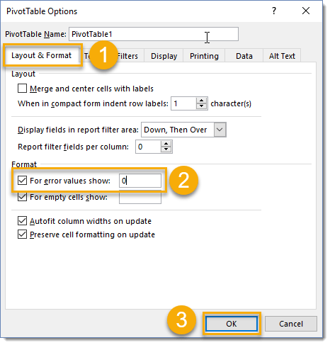
Enable fault values option.
- Go to the Layout & Format tab.
- Cheque the For error values show box and input a value or some text.
- Printing the OK button.
Now your pivot tabular array will be much more than presentable.
Add Relationships to Between Tables
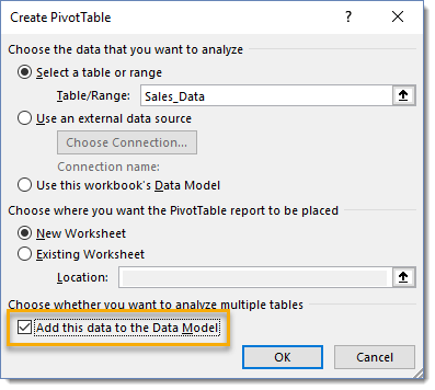
You can create relationships between different data tables using pin tables and the Data Model. When creating a pivot table bank check the Add this to the Data Model box in the Create PivotTable window.
For example if our sales data only contained a customer ID and the customers proper noun was stored in some other table, this would permit us to chronicle the customer ID to the proper noun and build sales data pivot tables based on the customer name.
Read this post for more item on building relationships in pivot tables.
Create a PivotChart
Pivot tables are astonishing, but even with a pivot table it's sometimes hard to see the trend or bibelot in the data. PivotCharts allow you to create a visualization of your pin table summary.
The cool matter is, they are dynamically linked together. If you change something in your pin table the changes will happen in your pivot chart and vise-versa.
Y'all can turn your pivot tables into a variety of different chart types.
- Column charts
- Line charts
- Pie charts
- Bar charts
- Area charts
- Radar charts
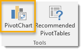
To insert a PivotChart select the pivot table you lot want to create PivotChart based on. Go to the Clarify tab in the ribbon and select PivotChart from the Tools section. Select the blazon of chart you want from the Insert Chart menu.
This can also be accessed from the Insert tab in the Charts section with the PivotChart control.
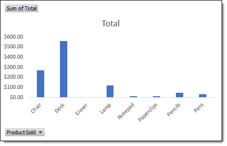
Now we take a visual representation of our pivot table! Y'all can use the field buttons in the chart (lower left corner in the higher up instance) to filter and sort your chart, notice this volition also update your pivot table!
Insert a PivotChart with a Keyboard Shortcut

Select a cell inside your pivot table and press Alt + F1 to quickly add together a PivotChart to the aforementioned sheet as your pivot table.
Y'all tin can use the alternate ribbon control shortcut keys of Alt + N + SZ
Add a Slicer
Slicers are peachy for making dynamic and interactive dashboards. They piece of work exactly like a filter but the list of filtered items will remain visible to the user.
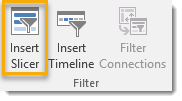
Go to the Analyze tab in the ribbon and select Insert Slicer under the Filter section.

Select the fields for which you want to create the slicer. Selecting multiple fields will effect in a separate slicer for each field selected.
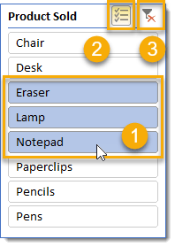
You tin now filter on any combination of items from your slicer.
- Select whatever item with a left click. You tin select multiple adjacent items with a left click and drag.
- Turn on multi-select mode to select multiple non-side by side items.
- Clear your selected filter and start again.
Add together a Timeline
To add together a Timeline to your pivot table or chart, your source data will need to contain a engagement field.
Timelines are exactly like Slicers, just just for utilise with engagement fields. They allow you to filter on dates with a visual fourth dimension line slider bar.
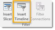
Become to the Clarify tab in the ribbon and select Insert Timeline under the Filter section.
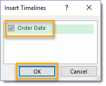
Select the appointment fields for which you desire to create the Timeline. Selecting multiple fields will result in a separate timeline for each field selected.
You tin now filter your data on any range of dates from your Timeline.
- Select to filter past Days, Months, Quarters or Years.
- Drag the end of the timeline to arrange the filtered range. Unfortunately, there is no multi-select like the slicers and you lot can only select ane continuous range of dates.
- Clear your filter to start again.
Hide All Field Buttons on a Pin Nautical chart
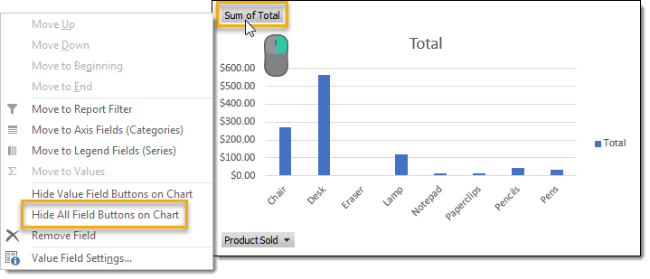
Generally speaking, having less junk on your charts is better! This is why I like to remove all the buttons on a PivotChart to free up valuable chart existent estate. Whatever filtering needed can be done from the linked pivot table instead of from the chart.
Right click on any of the buttons on the chart and select Hibernate All Field Buttons on Chart.
Connect Slicers or Timelines to Multiple Pivot Tables
You can connect your slicers and timelines to any number of pin tables. This means you tin control many pivot tables or pin charts from ane single slicer or timeline. This is bully for creating interactive dashboards.
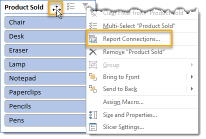
Right click on the slicer or timeline and then select Written report Connections from the menu. You lot tin can also access this from the Slicer Tools Choice ribbon tab when your slicer is selected.
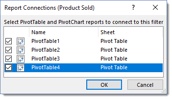
Select whatsoever pivot tables you desire to connect to the slicer past checking the respective box and printing the OK button. This is where properly naming your pin tables can really pay off.
Change the Number of Columns in a Slicer
If your field has a lot of items in it, you can conserve some space while still showing all items in the slicer by adjusting the number of columns.

Right click on the slicer and then select Size and Backdrop from the carte.
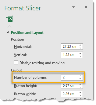
In the Format Slicer window under the Position and Layout section prepare the desired Number of columns.
At present yous can fit the same number of items in a smaller expanse within your slicer.
Filter on Top N Items

Yous can add filters to show your top or lesser N from your pivot table.

From the filter icon, go to the Value Filters section and select Summit ten. You volition exist able to select from a variety of options.
- Select to either bear witness the Elevation or Bottom results from your pivot table.
- Select a number of items, percentage or full sum for the top or lesser criteria.
- Select from either Items, Per centum or Sum.
- Items – This volition show the items in your field that have the highest or everyman N values.
- Pct – This will show the items in your field where the value is in the peak or bottom Nth percentile.
- Sum – This will prove the top or lesser items in your field where the sum is greater than the number entered in stride ii.
- Select the metric in your pin tabular array values surface area to base of operations the top or bottom results on.
Add together a Value Filter for any Field
Nosotros can filter any field in the row or column area of a pivot tabular array based on the associated value in the values surface area.
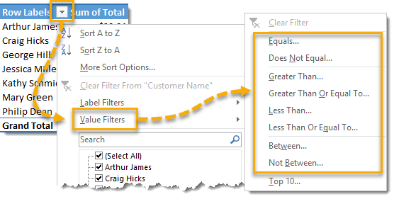
Click on the filter icon to the right of the field name. Select Value Filters from the menu. From here you tin can select any number of options.
- Filter on items where the value Equals a given value.
- Filter on items where the value Does Non Equal a given value.
- Filter on items Greater Than a given value.
- Filter on items Greater Than Or Equal To a given value.
- Filter on items Less Than a given value.
- Filter on items Less Than Or Equal To a given value.
- Filter on items Betwixt two given values.
- Filter on items Non Between ii given values.
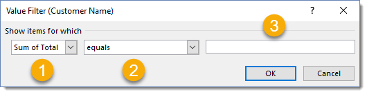
Regardless of which value filter selection you selected, you lot'll be able to arrange it from the value filters criteria menu.
- Select which values field your criteria volition apply to.
- Select the filtering choice desired. This allows you to alter the pick you previously selected.
- Enter the criteria value to filter based on. If y'all selected a filtering selection that requires two inputs, at that place volition be ii input fields here.
Increase the Row Label Indent in Compact Form Layout
You tin increase the indent for row labels in a compact form layout pin table to add together a chip more of a distinct separation between fields.
Select your pivot table and go to the Clarify tab and select Options.
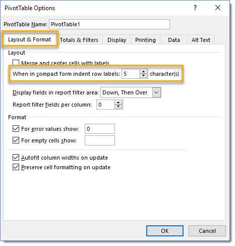
Go to the Layout & Format tab then adjust the graphic symbol count for your indent as desired.
Add Multiple Subtotal Calculations
When you add together subtotals to your pivot table, past default information technology will but show the sum subtotal. It is possible to alter this to show a different adding like Count, Average, Minimum, Maximum, Standard Deviation and others. It's too possible to show multiple different subtotal calculations at the same fourth dimension!
For this, you'll need to take a pivot tabular array with at least two fields in the rows area of the pin table.
Correct click on the field you're going to add together unlike subtotals to and then select Field Settings from the menu.

From the Field Settings menu nether the Subtotals & Filters tab select the Custom subtotals option then select any Subtotal Adding type.
This is an crawly way to show more summary information in your pivots.
Include New Items in Manual Filters

Let's say you've spent a decent amount of time manually filtering your pivot table to a select number of field items.
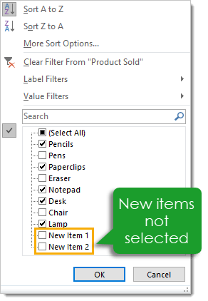
Y'all then add together information to your source data gear up and the new data contains additional items in your field which weren't in the previous data.
When you refresh your pivot table, the new information items volition not be included in the filtered items. You accept to go through and manually select those new items if you want them to appear in the filtered pivot tabular array.
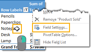
You can change this so that new information items in a field are automatically added to any transmission filters. Correct click on the field then select Field Settings.
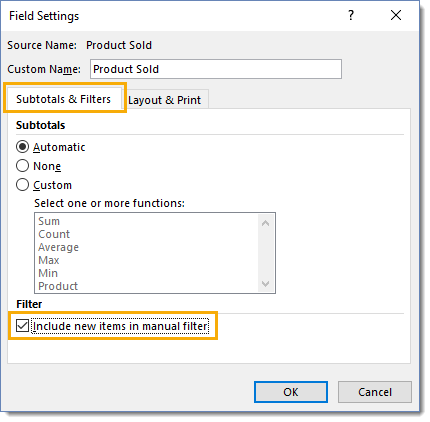
From the Field Settings menu go to the Subtotals & Filters tab and check the Include new items in transmission filter box.
Apply an External Data Connection Source
You can use an external data source for your pivot tabular array. This means you can store your data in another Excel file or CSV and practice your analysis in a dissever workbook. Your information can be updated by other people or systems without affecting your electric current workbook and assay.
Select the cell where you desire your new pin table to announced then go to the Insert tab in the ribbon and select PivotTable from the Tables section.
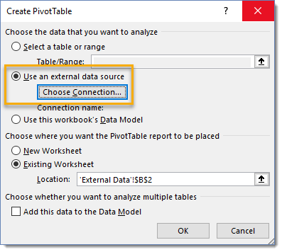
From the Create PivotTable menu select the Use an external data source radio button then click on the Choose Connection push button.
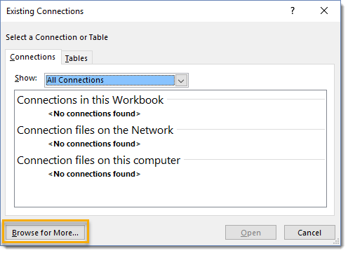
In the Existing Connection carte du jour select Browse for More than. In the resulting file picker menu, navigate to the desired file and select it so printing the Open up button.
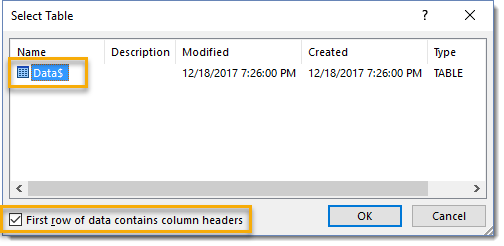
In the resulting select table menu select the location of the information from your file. My data was in a tabular array on a sheet called Data so I have selected Data$ from the list. Make sure to check the Starting time row of data contains column headers box if your data has column headers and then press the Ok button.
Y'all tin now finish creating and building your pivot table as usual.
Refresh External Connections on a Schedule
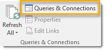
Yous can set your external connections to refresh with any new or updated data on a periodic schedule of your choosing. Become to the Information tab in the ribbon and select the Queries & Connections command.
If you select the pin table with your external connection first, you tin can directly open the Properties menu from the Data tab.
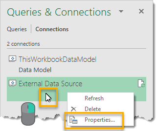
Correct click on the external connection from the Queries & Connections window and select Backdrop from the bill of fare.
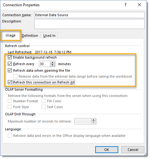
Under the Usage tab in the Connection Properties menu, cheque the Refresh every N minutes box and then set the number of minutes.
Note that all the Refresh command options are disabled (unchecked) past default. You can also enable a few other options from this menu.
- Enable background refresh
- Enable Refresh data when opening the file
- Enable Refresh this connection on Refresh All
Show Value As
The side by side 10 tips are the among the most powerful features of pivot tables, however nigh Excel users don't know almost them.
At some stage you've probably gone off to the side of your pivot table and done some formula calculations to run across how much of a percentage a value represents, calculated a running total or a pct difference. This stuff is already a baked in feature known every bit Show Values As.
Unfortunately it'due south sort of subconscious in the right click menu or equally the secondary tab in the Value Field Settings. It's and then useful and powerful information technology really deserves a featured spot in the Clarify tab of the ribbon.
Yous can access this feature a couple of dissimilar ways.
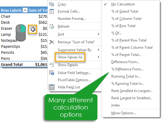
Right click on any value and then select Prove Values As from the card. In the sub-carte du jour you'll be able to select from many dissimilar calculation options. You'll besides be able to set a field back to No Calculation from here.
Another choice is to access this through the Value Field Settings card.
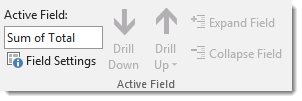
Become to the Analyze tab and press the Field Settings button found under the Agile Field section.
Or you can right click anywhere on the field to open the bill of fare and so select Value Field Settings.
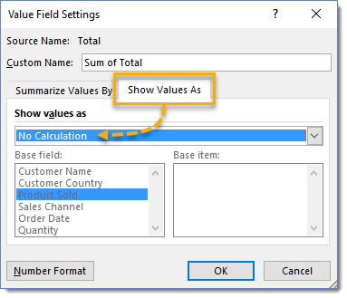
In one case you're at the Value Field Settings menu go to the Prove Values As tab.
There are many options hither as to how to display your values. We'll explore these in the post-obit tips.
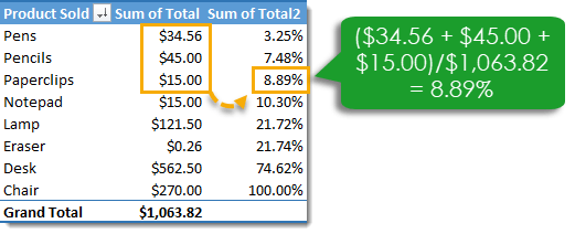
Show Value as % of 1000 Full

Select the % of Yard Total option to show all values as a per centum of the yard total. When selected the 1000 Full volition bear witness equally 100% and all the values in the Value area will add together up to 100%.
Evidence Value as % of Column Total
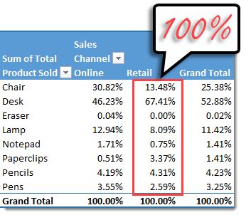
Select the % of Column Total option to testify all values in each column as a pct of that columns full. When selected each cavalcade total will show as 100% and all the values in each cavalcade will add together upwardly to 100% including the Chiliad Total column.
Show Value every bit % of Row Total
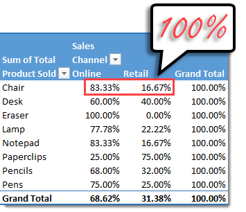
Select the % of Row Total option to show all values in each row as a percentage of that rows full. When selected each row total will show every bit 100% and all the values in each row will add up to 100% including the Grand Total row.
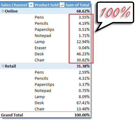
Evidence Value equally % of Parent Cavalcade
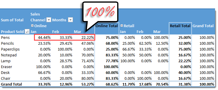
Select the % of Parent Cavalcade option to show all values in each row as a percent of its parent column. Each row of values within a parent column will add together to 100%. The 1000 Total column will contain all 100% values.
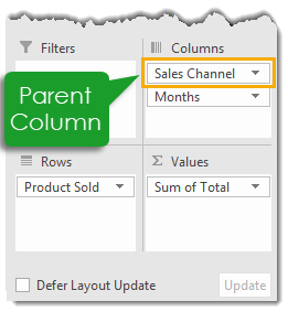
A parent cavalcade volition exist the top most field in the Columns area of the pivot table.
Testify Value as % of Parent Row
Select the % of Parent Row pick to prove all values in each cavalcade as a pct of its parent row. Each column of values inside a parent row will add to 100%. The K Full row volition incorporate all 100% values.
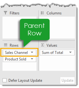
A parent row volition exist the superlative nigh field in the Rows area of the pivot table.
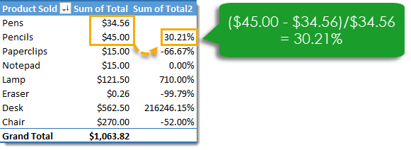
Show Value as Difference
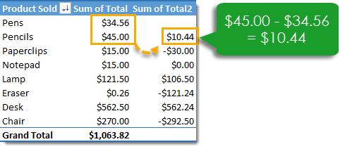
Select the Divergence From option to show all values every bit the departure between the current particular and previous item, side by side item or a fixed detail'southward value.
Testify Value as % of Difference
Select the % Difference From pick to evidence all values as the pct departure betwixt the current detail and previous item, next item or a fixed detail's value.
Show Value as Running Total
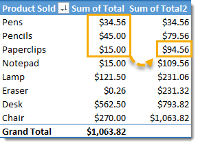
Select the Running Total In choice to show a running full for a given field.
Bear witness Value as % of Running Total
Select the % Running Full In pick to prove the running full for a given field as a percent of the Grand Total.
Prove Value as Rank
Select the Rank Smallest to Largest or Rank Largest to Smallest option to testify a fields rank.

I Have 40 Columns Of Raw Data, How To Create A Template To Grab 10 Of Them?,
Source: https://www.howtoexcel.org/pivot-table-tips-and-tricks/
Posted by: schellfromen.blogspot.com
0 Response to "I Have 40 Columns Of Raw Data, How To Create A Template To Grab 10 Of Them?"
Post a Comment